Predictive modeling for assessing automobile insurance risks
Introduction
The automobile industry has always been at the forefront of innovation, constantly seeking ways to improve efficiency, safety, and customer satisfaction.
Predictive modeling adds a new dimension to this effort by enabling data-driven decisions that benefit manufacturers, insurers, and consumers.
In this project, we focus on predicting normalised losses for vehicles, a crucial metric for assessing automobile risk and determining insurance premiums.
Normalised losses are standardised metric that quantifies the relative risk of a vehicle incurring insurance losses.
This article leverages various machine learning models to provide accurate and actionable predictions.
Automobile insurance dataset
Normalised losses are typically calculated based on certain important data such as historical claims data, adjusted to account for varying factors such as repair costs, vehicle features, and accident frequency.
This allows for consistent comparison across different car models.
The dataset comprises 206 rows and 26 columns, offering comprehensive insights into various vehicles. It includes technical specifications, insurance risk ratings, and normalised loss values, providing a robust foundation for analysis.
To access the dataset please visit the following link, which includes an in-depth article detailing a prior exploratory analysis conducted on the automobile dataset.
Aim of predictive modelling
In this project, we aim to predict normalised losses using various machine learning models, including Linear Regression, Ridge Regression, ElasticNet, Random Forest, Gradient Boosting, and Support Vector Machines (SVM).
The main steps to achieve this aim include:
- Data Preprocessing
- Model Selection
- Model Evaluation
- Hyperparameter tuning
- Feature Importance
Data Preprocessing
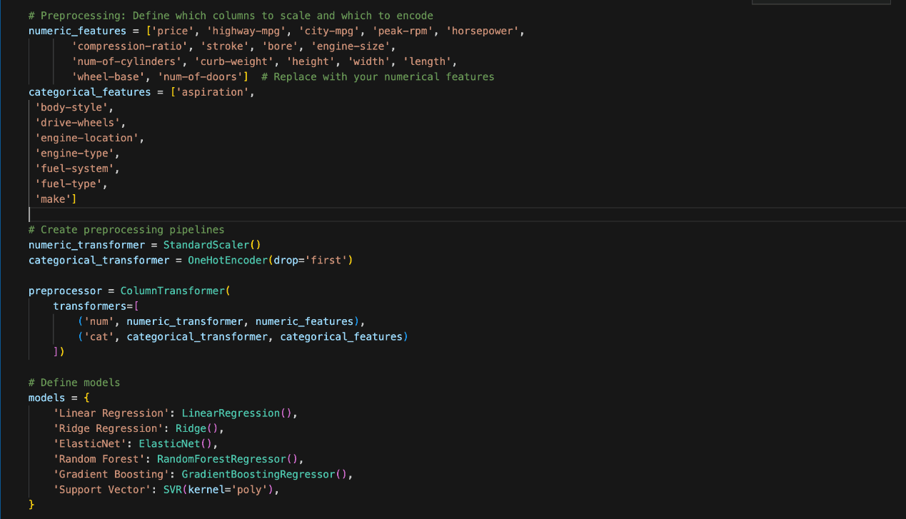
Preprocessing is essential for preparing the dataset before applying machine learning models. The Python coding in the figure below was used.
The features were divided into two categories, namely Numeric and Categorical.
The numeric features include values such as ‘price’, ‘horsepower’, and ‘engine-size’. We scaled them using StandardScaler to ensure all numeric variables have the same weight when fed into the models.
On the other hand, the categorical or non-numeric features include ‘aspiration’, ‘body-style’, and ‘fuel-type’.
Categorical data was transformed using OneHotEncoder, which converts them into binary columns with 1 representing the presence and 0 representing the absence of each category.
Model Selection
Several algorithms can be utilised in the prediction of normalised losses in the automobile insurance business.
However, the performance of these algorithms will vary depending on the nature of the dataset and the specific problem to be tackled.
Therefore, it is important to try out multiple algorithms and compare them based on certain evaluation criteria to select the best one while also aiming to balance complexity and interpretability.
Below are the algorithms considered and explored.
1. Linear Regression
Linear Regression is one of the simplest machine learning models. It tries to find a straight line (or hyperplane) that best fits the data.
The idea is that the target variable ‘y’ (like ’normalised-loss’`) can be expressed as a linear combination of the input features ‘x’ (like’`price’,’`horsepower’, etc.). Learn more about Linear Regression here.
The goal of Linear Regression is to minimise the error between the predicted and actual values. The error is measured using the mean squared error (MSE).
2. Ridge Regression
Ridge Regression is like Linear Regression but with a penalty for large coefficients (weights). This helps prevent overfitting.
Math is almost the same as Linear Regression, but it adds a regularisation term that penalises large weights.
Learn more about Ridge Regression here.
3. Random Forest Regressor
Random Forest is an ensemble method that combines multiple Decision Trees. A decision tree splits the data into smaller groups, learning simple rules (like “if price > 10,000, predict high loss”).
A Random Forest builds many decision trees and averages their results. The randomness comes from:
– Selecting a random subset of data for each tree.
– Using random subsets of features at each split.
Each tree makes its own prediction, and the final result is the average of all tree predictions.
Important concepts:
– Splitting Criteria: In regression, trees are usually split by minimising the mean squared error (MSE).
– Bagging: This means each tree is trained on a random subset of the data, which makes the forest more robust.
More about Random Forest here.
4. Gradient Boosting Regressor
Gradient Boosting is another ensemble method that builds decision trees. However, unlike Random Forest, each tree learns from the mistakes of the previous one. It works by fitting trees sequentially.
The first tree makes predictions, and the next tree focuses on correcting the errors made by the previous tree.
Learn about Gradient Boosting Regressor here.
5. Support Vector Regressor (SVR)
Support Vector Regressor tries to find a line (or hyperplane) that best fits the data, but instead of minimising the error for all points, it allows a margin of error. SVR uses a boundary where it doesn’t care about errors (a margin).
SVR tries to balance minimising errors and keeping the model simple by only adjusting predictions outside this margin.
6. ElasticNet
ElasticNet combines the ideas of Lasso Regression and Ridge Regression. Like Ridge, it penalises large coefficients but also like Lasso, it can reduce some coefficients to zero, making it useful for feature selection.
ElasticNet is good when you have many features and want both regularisation and feature selection.
Model Evaluation
Some of the more commonly known model evaluation methods or metrics used in this project are RMSE, MSE, and R-squared.
Splitting the dataset into training and test sets is an evaluation method used before the first model is even built.
By setting aside a portion of the data as the test set, we ensure that the model is evaluated on unseen data, providing an early and unbiased estimate of how well the model will generalise new data.
After experimenting with different algorithms using the test split ratio, the following performance metrics were used to compare the regression models on an equal footing:
Mean Squared Error (MSE):
MSE measures the average squared difference between the actual and predicted values.
A lower MSE indicates a better fit, but it’s sensitive to outliers.
Root Mean Squared Error (RMSE):
The RMSE is the square root of MSE, and it’s useful because it’s in the same units as the target variable.
Mean Absolute Error (MAE):
MAE measures the average absolute difference between the actual and predicted values.
It’s less sensitive to outliers than MSE.
R-squared (R²):
R² explains how much of the variance in the target variable is captured by the model.
A higher R² (closer to 1) indicates a better fit, but it’s not always reliable for small datasets.
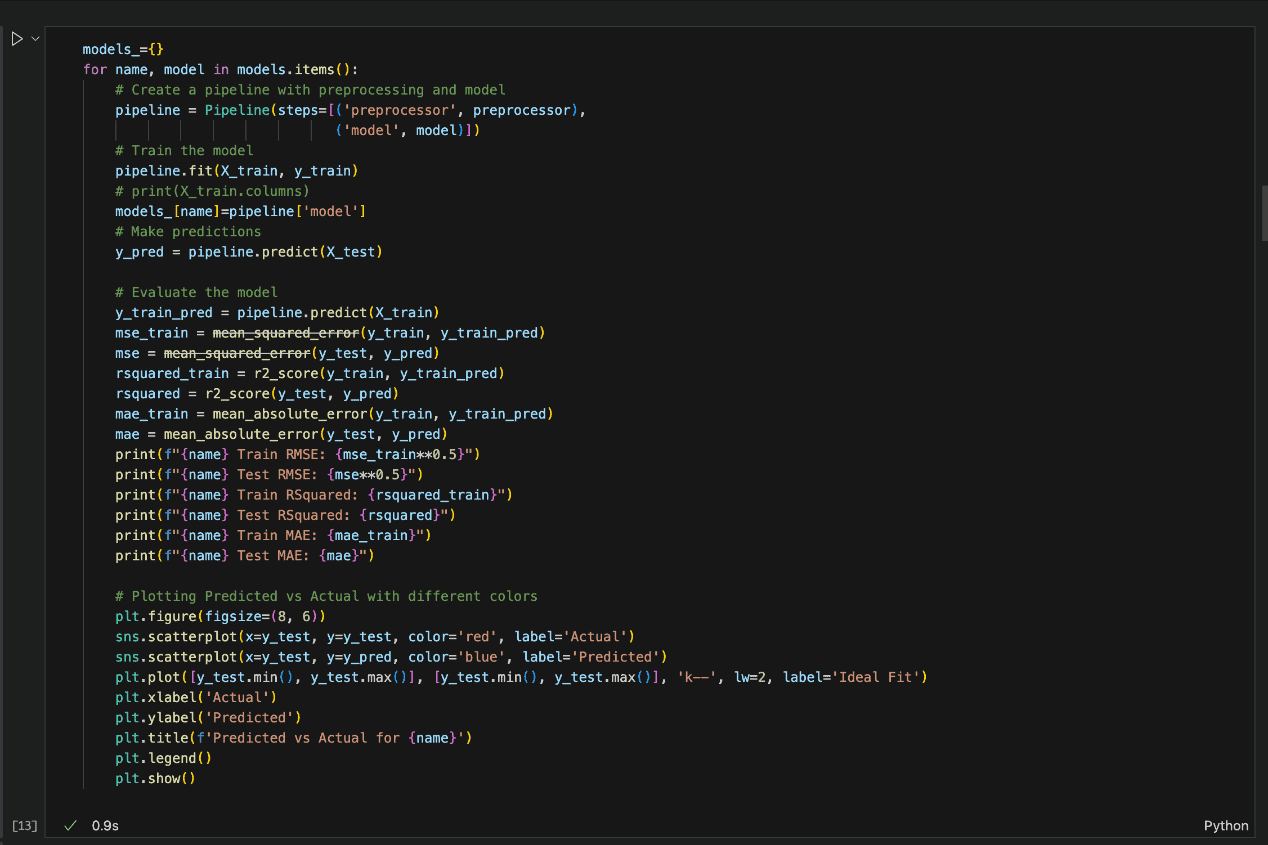
In the snapshot of the Python code below, each of the model algorithm and the evaluation method is implemented.
Results
The following table summarises the results of the different models used based on RMSE, MAE, and R-squared values:
Models | RMSE | MAE | R-squared |
Linear Regression | 16.4 | 13.9 | 80.5 |
Ridge Regression | 23.4 | 17.7 | 60.3 |
Random Forest Regressor | 26.8 | 18.4 | 48.2 |
Gradient Boosting Regressor | 23.5 | 15.1 | 60.0 |
Support Vector Regressor | 36.7 | 33.9 | 2.8 |
Elastic Net | 28.7 | 25.6 | 40.4 |
From the results presented, Linear Regression seems to demonstrate the best overall performance compared to the other models, followed by Gradient Boosting Regressor and Random Forest.
However, it could be observed that the tree-based models (Random Forest and Gradient Boosting Regressor) may be exhibiting signs of overfitting.
While their training performance is near perfect, their test performance is significantly worse, indicating that these models may not generalize well to unseen data.
Models | RMSE train | RMSE test | MAE train | MAE test | R-Squared train | R-Squared test |
Random Forest Regressor | 6.9 | 26.8 | 4.3 | 18.4 | 96.1 | 48.2 |
Gradient Boosting Regressor | 4.1 | 23.5 | 3.1 | 15.1 | 98.6 | 60.0 |
Hyperparameter Tuning
Choosing the right hyperparameters can significantly improve the model’s performance and its ability to generalise to unseen data. If the hyperparameters are not tuned correctly:
- The model might overfit (perform well on training data but poorly on test data).
- The model might underfit (fail to capture the patterns in the data).
How to Perform Hyperparameter Tuning
- Manual Search: You manually try different combinations of hyperparameters and evaluate performance. This approach can be time-consuming and inefficient.
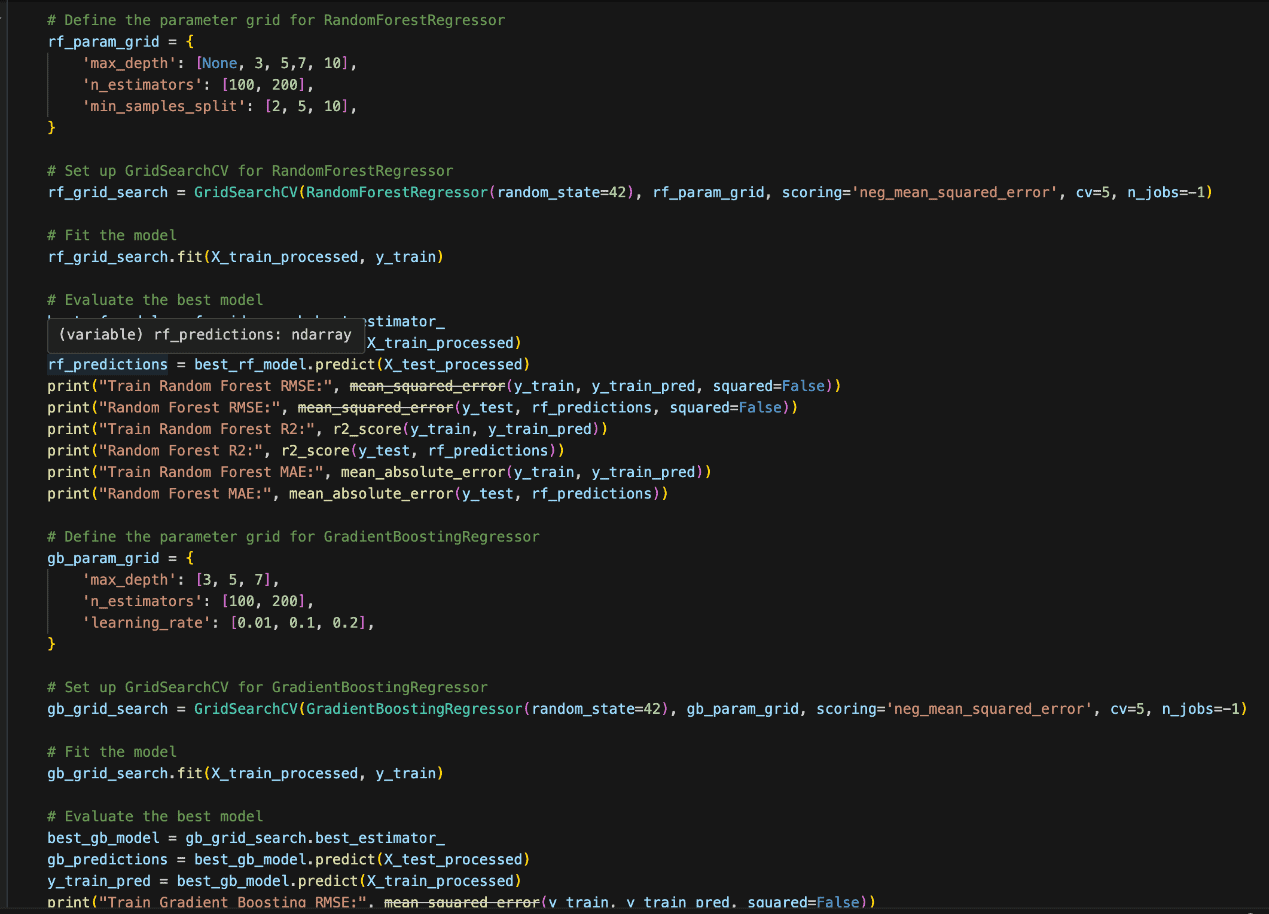
- Grid Search: You define a set of hyperparameter values to try, and the algorithm tries every combination. It’s exhaustive but computationally expensive, especially when the search space is large.
Since we have a relatively small sample size, we will be using grid search as seen in the Python code snippet below:
Results after tuning
Models | RMSE train | RMSE test | MAE train | MAE test | R-Squared train | R-Squared test |
Random Forest Regressor | 8 | 25.2 | 5.7 | 19.3 | 94.8 | 54.1 |
Gradient Boosting Regressor | 5.1 | 21.9 | 3.8 | 15.2 | 97.9 | 65.8 |
Even though the training scores for the tree-based models have decreased and the test scores have improved, the gap between the two still indicates signs of overfitting.
This suggests that, despite the adjustments, the models struggle to generalise.
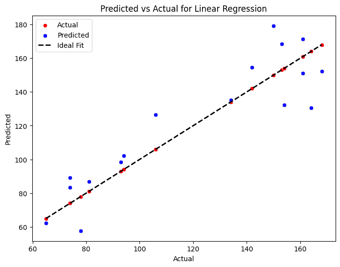
Overall, Linear Regression remains the top-performing model, showing no signs of overfitting and delivering strong, balanced results across both training and test datasets.
Feature Importance
To further enhance the interpretability of your model, it’s essential to understand which features contribute the most to the final predictions.
The method for evaluating feature importance varies by model type. For tree-based models like Random Forest or Gradient Boosting, we could utilise the built-in feature importance method.
For Linear Regression, the model’s coefficients can be analysed. Larger absolute values indicate features that have the most significant impact on the model’s predictions.
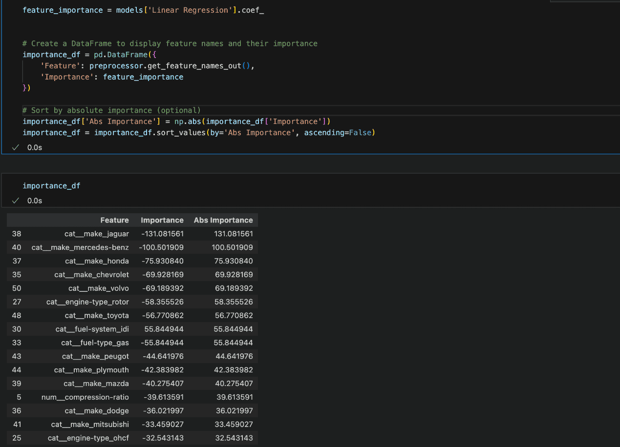
The feature importance reveals that the categories transformed into features through one-hot encoding have the largest coefficients.
This suggests that these categorical variables, once split into binary columns, have a significant influence on the model’s predictions.
It’s common in such cases for certain categories within a feature to carry more weight, especially if they represent distinct patterns or behaviors that strongly impact the outcome.
However, it’s important to carefully interpret these results, as large coefficients don’t necessarily mean the feature is inherently important—just that it has a stronger relationship with the target in the given model.
Model Interpretability using SHAP
Another method of calculating feature importance is by using SHAP.
SHAP (SHapley Additive exPlanations) is a powerful feature importance tool that uses cooperative game theory to assign each feature an importance value based on its contribution to a model’s predictions.
By computing Shapley values, SHAP quantifies how much each feature influences the output for individual predictions, enabling a clear understanding of model behavior.
To calculate feature importance using SHAP, this method can be followed:

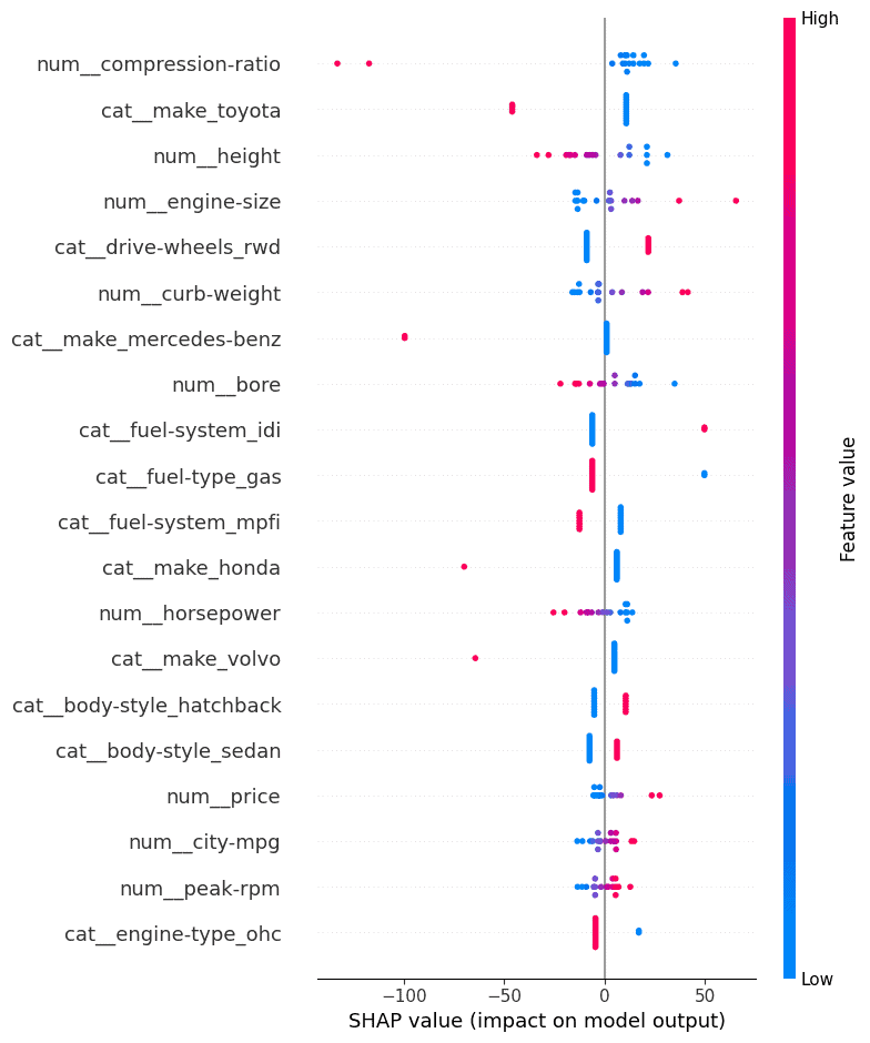
The SHAP plot displayed below shows the importance of different features on the model’s predictions. The SHAP values on the x-axis indicate the extent to which each feature influences the model’s output, with positive or negative contributions.
The further the SHAP value is from zero, the stronger the feature’s impact on the prediction. The colors represent the feature values: blue for low values and pink for high values.
Key Observations:
- Compression-ratio (num__compression-ratio) has the most significant impact, with higher values (in pink) increasing the SHAP values and positively influencing the model’s predictions. Conversely, lower compression ratios (in blue) push the prediction in the negative direction.
- Make Toyota (cat__make_toyota) also has a strong influence. High SHAP values suggest that cars of this make contribute positively to the model’s outcome.
- Height (num__height) shows a clear trend where higher values contribute positively, and lower values push predictions downward.
- Engine size (num__engine-size) and curb weight (num__curb-weight) are among the top features, with larger engines and heavier vehicles generally contributing to higher predictions. This aligns with expectations, as these attributes often correlate with vehicle performance.
- Make Mercedes-Benz (cat__make_mercedes-benz) have a distinct effect, with higher SHAP values driving the prediction positively, reflecting its luxury status.
- The drive wheels (cat__drive-wheels_rwd) feature, particularly rear-wheel drive cars, tend to influence predictions positively when rear-wheel drive is present.
- This SHAP analysis reveals that some of the most influential features are related to vehicle specifications (engine size, curb weight, height) and specific car make (Toyota, Mercedes-Benz).
Business implications of car insurance risk prediction results
- Insurance Premium Calculation: By predicting normalized losses, insurance companies can more accurately set premiums for different car models. Cars with higher predicted normalized losses would be considered riskier, leading to higher premiums, and vice versa.
- Risk Assessment for New Car Models: Car manufacturers or dealers could use this model to assess the insurance risk rating of new or upcoming car models. This helps in evaluating how risky it might be to insure the car based on its features and the history of similar vehicles.
- Accident/Claim Risk Prediction: Predicting normalised losses could indicate how prone a car is to accidents or damage based on features like engine size, horsepower, or body type, allowing manufacturers or consumers to assess the likelihood of incurring future repair costs.
- Vehicle Rating Systems: Predicting normalized losses can contribute to a more comprehensive vehicle rating system for buyers, helping them make informed decisions about the long-term costs of owning a particular car, including insurance expenses.
Wrapping up
In summary, this project demonstrates the power of predictive modeling in estimating normalised losses for vehicles.
Among the models tested, Linear Regression emerged as the top performer, striking an effective balance between accuracy and simplicity.
Advanced models like Random Forest and Gradient Boosting, while promising, exhibited challenges with overfitting, underscoring the importance of careful model tuning and evaluation.
The analysis also highlighted the critical features influencing predictions, such as engine size, curb weight, and specific car make, providing actionable insights for stakeholders.
By leveraging these models, insurance companies can optimise premium pricing, manufacturers can assess risk ratings for new models, and consumers can make more informed vehicle purchase decisions.
This approach exemplifies how machine learning can bridge the gap between complex data and practical, real-world applications.


