How to predict financial fraud using Python

The dataset for this analysis can be downloaded from GitHub using this link and kaggle. The Python code for the analysis can be downloaded here.

Overview of the financial fraud dataset

The dataset consists of 14,446 rows and 15 columns, with the following structure:

1. Date and Time Features:
   • trans_date_trans_time: Timestamp of the transaction.
     
2. Transaction and Location Features:
   • merchant: The name of the merchant where the transaction occurred.
   • category: The category of the transaction, such as grocery_net, shopping_net, etc.
   • amt: The amount of money spent in the transaction.
   • city and state: The location where the transaction took place.
   • lat and long: Latitude and longitude of the transaction location.
   • merch_lat and merch_long: Latitude and longitude of the merchant’s location.
     
3. Demographic and Personal Features:
   • city_pop: The population of the city where the transaction took place.
   • job: The job title of the individual making the transaction.
   • dob: The date of birth of the individual, currently in object format.
   • trans_num: A unique identifier for the transaction.
     
4. Target Variable:
   • is_fraud: Indicates whether the transaction was fraudulent (1) or not (0).

Step-by-step analysis of financial fraud

1. Data Cleaning and Preprocessing:

• Convert trans_date_trans_time to datetime format.
• Convert dob to datetime format and calculate the age of the individual at the time of the transaction.
• Convert is_fraud from an object to an integer for easier analysis.

2. Exploratory Data Analysis (EDA):

• Univariate Analysis: Analyse the distribution of the key variables such as amt, city_pop, and age.
• Bivariate Analysis: Explore the relationship between amt and other features like category, city_pop, and is_fraud.
• Geospatial Analysis: Plot the geographic distribution of transactions and identify any patterns related to fraud.

3. Analysis of Fraudulent Transactions using Machine learning

Feature engineering:

• Create additional features such as transaction_hour, transaction_day_of_week, and transaction_month from the trans_date_trans_time.
• Calculate the distance between the transaction location (lat, long) and the merchant’s location (merch_lat, merch_long).

Predictive modelling:

• Compare the distribution of features in fraudulent vs. non-fraudulent transactions.
• Identify key indicators of fraud based on the dataset.

4. Further Analysis

• Visualise the distribution of transaction amounts, the age distribution of customers, and the geographic distribution of fraud.
• Use box plots, histograms, and scatter plots to understand relationships and outliers.

STEP 1. Data Cleaning and Preprocessing:

The following Python script would clean and transform the data and make it ready for analysis by:

• Converting trans_date_trans_time to datetime format.
• Converting dob to datetime format and calculate the age of the individual at the time of the transaction.
• Converting is_fraud from an object to an integer for easier analysis.
  

# Data Cleaning and preprocessing
df['trans_date_trans_time'] = pd.to_datetime(df['trans_date_trans_time'], format='%d-%m-%Y %H:%M')
df['dob'] = pd.to_datetime(df['dob'], format='%d-%m-%Y')
df['age'] = df['trans_date_trans_time'].dt.year - df['dob'].dt.year
df['is_fraud'] = df['is_fraud'].str.extract('(\d)').astype(int)

STEP 2. EDA.

Univariate analysis:

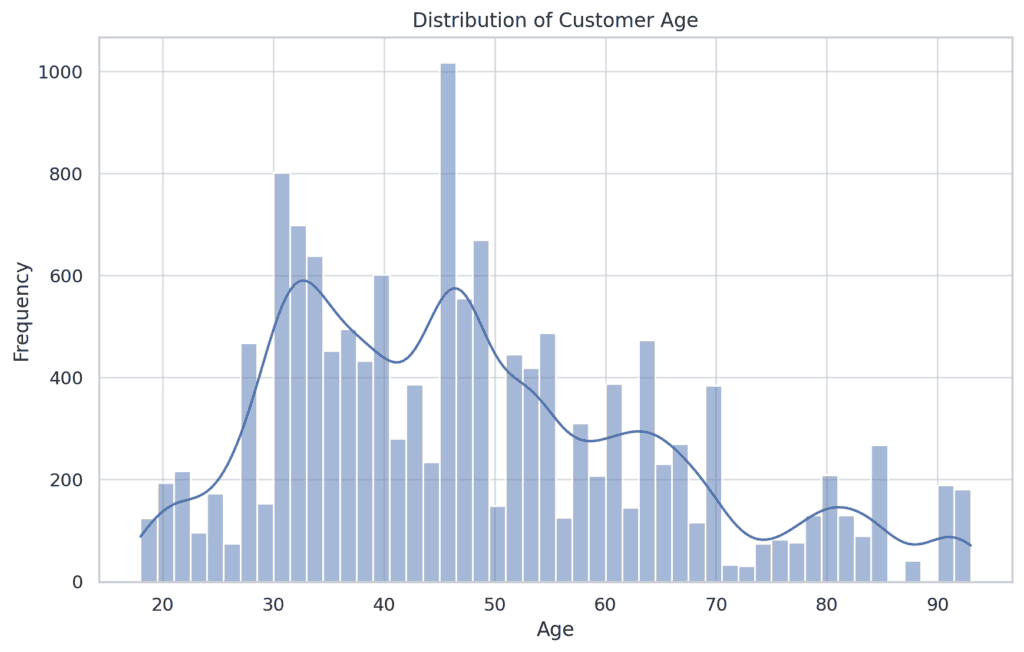
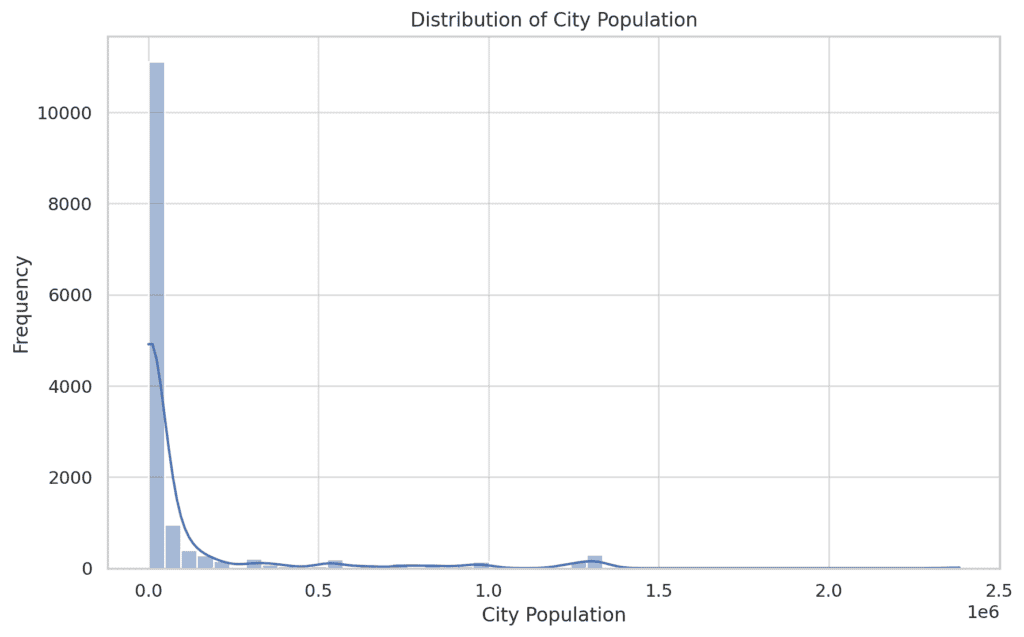
We’ll start with a univariate analysis to understand the distribution of key features like amt, age, and city_pop.

The univariate analysis reveals the following insights:

• Transaction Amounts:

The distribution of transaction amounts is right-skewed, with most transactions being relatively small. A few transactions have significantly higher amounts, indicating potential outliers.

• Customer Age:

The age distribution shows a concentration of customers in the middle age range, with fewer younger and older customers. This distribution appears to be slightly left-skewed.

• City Population:

The city population distribution is heavily right-skewed, indicating that most transactions occur in smaller cities, with a few taking place in larger cities.

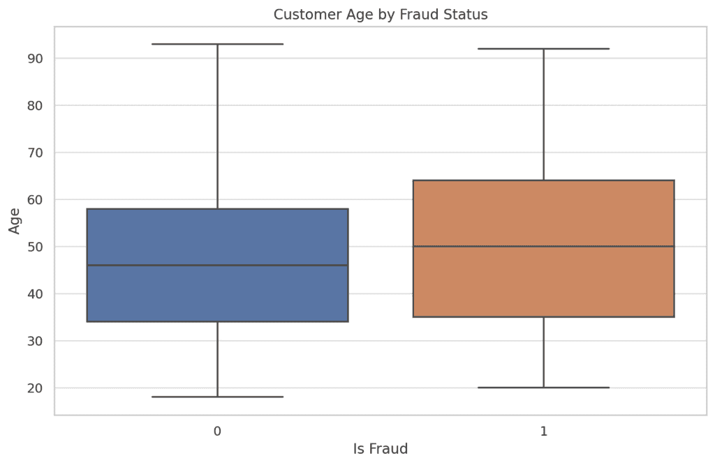
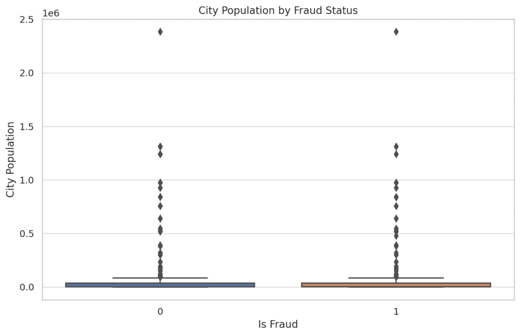
Bivariate Analysis:

We will perform a bivariate analysis to explore the relationships between key variables and the target variable (is_fraud).

This will include examining how the transaction amount, customer age, and city population relate to fraudulent activity.

The bivariate analysis provides the following insights:

• Transaction Amount vs. Fraud:

Fraudulent transactions tend to have higher amounts compared to non-fraudulent transactions. This suggests that high transaction amounts could be a potential indicator of fraud.

• Customer Age vs. Fraud:

The age distribution for fraudulent transactions does not significantly differ from non-fraudulent ones. This indicates that age might not be a strong predictor of fraud in this dataset.

• City Population vs. Fraud:

Fraudulent transactions are more likely to occur in cities with smaller populations. This could imply that fraudsters might be targeting less populated areas, possibly due to less stringent security measures.

Geospatial Analysis:

We will conduct a geospatial analysis to visualize the geographic distribution of transactions and identify any patterns related to fraud. ​

The geospatial analysis reveals the following:

• Geographic Distribution of Fraud:

Fraudulent transactions (marked in red) are spread across various locations, but there seems to be a concentration in certain areas.

This suggests that fraud activity might be more prevalent in specific regions, which could be worth further investigation.

• Comparison with Non-Fraudulent Transactions:

Non-fraudulent transactions (marked in blue) are distributed more evenly across the map. The overlap between fraudulent and non-fraudulent transactions indicates that fraud does not exclusively occur in isolated areas but rather within regions of regular transaction activity.

STEP 3. Analysis of Fraudulent Transactions using machine learning.

Feature Engineering:

First, we will refine and create additional features that could improve the predictive power of our model. We’ll then build and test a predictive model to identify fraudulent transactions.

We’ll create the following additional features which are relevant to the analysis using the following Python code:

• Transaction Frequency: The number of transactions made by a user in a given timeframe (e.g., daily, weekly).
• Merchant Consistency: The frequency of transactions at the same merchant by the same user.
• Distance Anomalies: The relationship between the distance of the transaction from the user’s home location and whether it was fraudulent.
• Transaction Hour: The hour when the transaction occurred.
• Transaction Day of Week: The day of the week when the transaction occurred.
• Transaction Month: The month when the transaction occurred.

# Feature Engineering
df['transaction_hour'] = df['trans_date_trans_time'].dt.hour
df['transaction_day_of_week'] = df['trans_date_trans_time'].dt.dayofweek
df['transaction_month'] = df['trans_date_trans_time'].dt.month

def calculate_distance(row):
    trans_location = (row['lat'], row['long'])
    merch_location = (row['merch_lat'], row['merch_long'])
    return geodesic(trans_location, merch_location).kilometers

df['distance_to_merch'] = df.apply(calculate_distance, axis=1)
df['daily_transaction_count'] = df.groupby(df['trans_date_trans_time'].dt.date)['trans_num'].transform('count')
df['merchant_consistency'] = df.groupby(['job', 'merchant'])['trans_num'].transform('count')

Predictive Modelling:

Next, we’ll use these features, along with the original ones, to build a predictive model.

We will use these Python script to do the following:

• Split the data into training and testing sets.
  
• Build a model (using Random Forest Classifier) to predict whether a transaction is fraudulent.
  
• Evaluate the model using appropriate metrics like accuracy, precision, recall, and F1-score.

# Model Building
features = [
    'amt', 'age', 'city_pop', 'distance_to_merch', 
    'daily_transaction_count', 'merchant_consistency',
    'transaction_hour', 'transaction_day_of_week', 'transaction_month'
]
X = df[features]
y = df['is_fraud']

X_train, X_test, y_train, y_test = train_test_split(X, y, test_size=0.3, random_state=42)
model = RandomForestClassifier(n_estimators=100, random_state=42)
model.fit(X_train, y_train)

y_pred = model.predict(X_test)
report = classification_report(y_test, y_pred)
conf_matrix = confusion_matrix(y_test, y_pred)
print(report)
print(conf_matrix)

The Random Forest model has produced the following results:

Precision:

• For non-fraudulent transactions (class 0): 100%
  
• For fraudulent transactions (class 1): 100%

Recall:

• For non-fraudulent transactions: 100%
  
• For fraudulent transactions: 99%

F1-Score:

• For non-fraudulent transactions: 100%
  
• For fraudulent transactions: 99%

Confusion Matrix:

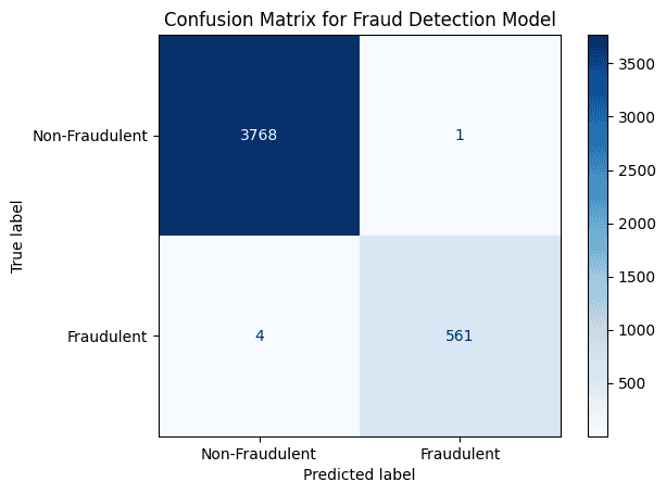
• True Positives (fraud detected correctly): 561
  
• True Negatives (non-fraud detected correctly): 3768
  
• False Positives (non-fraud detected as fraud): 1
  
• False Negatives (fraud not detected): 4

Report Interpretation:

• The model performs exceptionally well, with nearly perfect precision, recall, and F1-scores.
  
• There are very few misclassifications, with only 1 non-fraudulent transactions incorrectly classified as fraud and 4 fraudulent transactions missed.
  

STEP 4. Further Analysis:

Financial Fraud by Category

Let’s examine the distribution of fraud across different transaction categories to identify which categories are more vulnerable to fraudulent activity.

The plot above reveals that certain transaction categories, such as shopping_net, grocery_pos, and misc_pos, exhibit a higher incidence of fraud compared to others.

This suggests that these categories might be more attractive or vulnerable to fraudulent activities.

Analysis of Financial Fraud by Time.

Analysing fraud by time can provide insights into when fraudulent activities are most likely to occur. We can explore fraud patterns by:

1. Hour of the Day: Understanding at which times of day fraud is more frequent.
   
2. Day of the Week: Identifying whether certain days have higher fraud occurrences.
   
3. Month of the Year: Looking at seasonal patterns in fraud activities.

The visualisations of fraud by time provide the following insights:

1. Fraud by Hour of the Day:

Fraudulent transactions are more frequent during certain hours, particularly late at night and early in the morning.

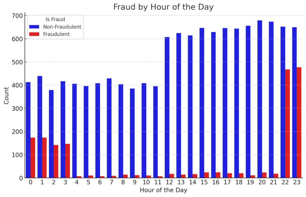
This might indicate that fraudsters prefer to operate when they expect lower monitoring or fewer security checks.

2. Fraud by Day of the Week:

Fraudulent transactions appear to be fairly evenly distributed throughout the week, with a slight increase on weekends.

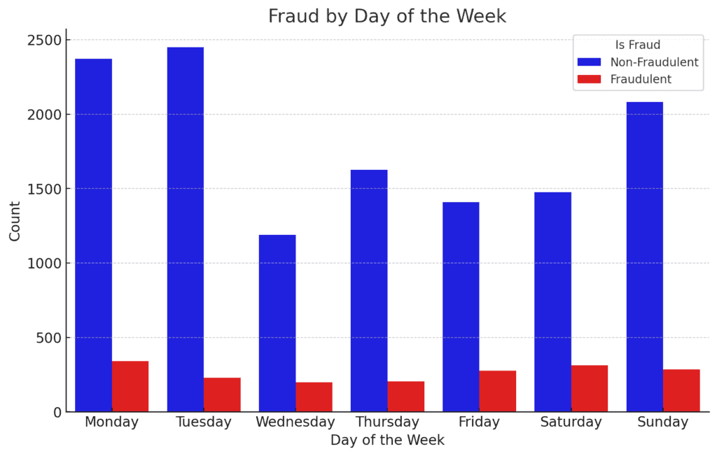
This could suggest that weekends might be a more opportunistic time for fraudsters, possibly due to reduced vigilance by financial institutions.

3. Fraud by Month of the Year:

The distribution of fraud across the months does not show a very strong seasonal pattern, though there are slight variations.

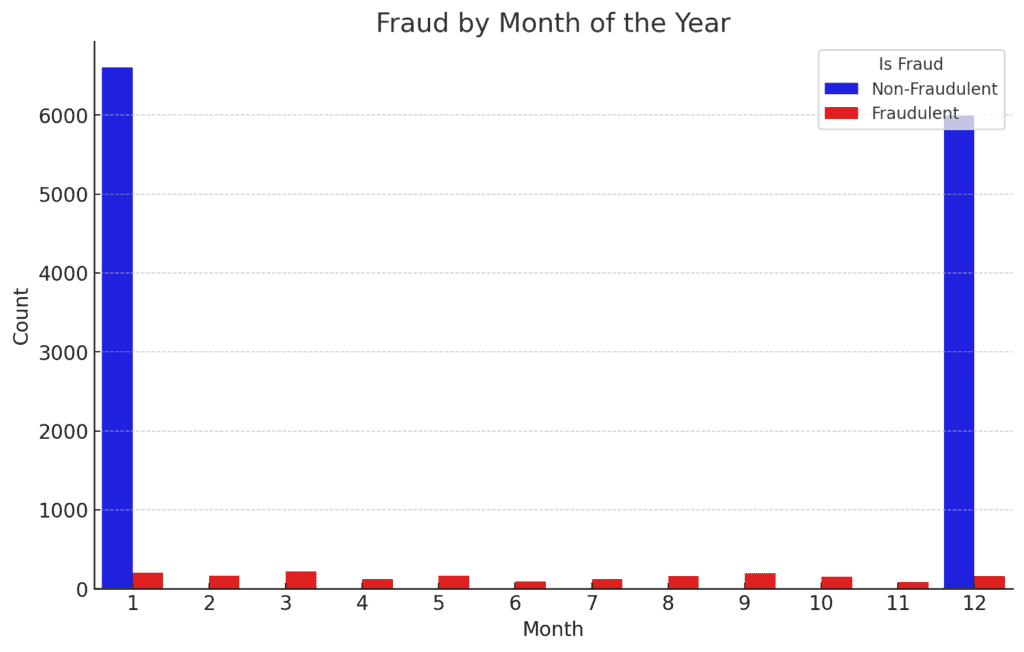
It might be interesting to investigate further if there are any specific events or holidays that correlate with these variations.

Conclusion

Through this comprehensive analysis, we have identified several key patterns associated with fraudulent transactions, including higher transaction amounts, specific transaction categories, and certain geographic locations.

Our machine learning model demonstrated strong performance in predicting fraud, and further optimization could enhance its accuracy even more.

By leveraging these insights, financial institutions can implement more targeted fraud prevention measures, ultimately reducing the risk of fraud and protecting both their assets and their customers.

This analysis serves as a foundation for building more sophisticated and adaptive fraud detection systems in the future.