How to predict income levels using machine learning

The dataset for this analysis can be downloaded from this GitHub link and here. The Python code for the analysis can be downloaded here.

Here’s a brief description of the columns:

1. age: The age of the individual.
   
2. workclass: The type of employer or self-employment status.
   
3. fnlwgt: Final weight, representing the number of people the observation represents.
   
4. education: The highest level of education attained.
   
5. education-num: The number corresponding to the education level.
   
6. marital-status: Marital status of the individual.
   
7. occupation: The type of job held by the individual.
   
8. relationship: The relationship of the individual to other members of the household.
   
9. race: The race of the individual.
   
10. sex: The gender of the individual.
    
11. capital-gain: Income from investment sources, apart from wages/salary.
    
12. capital-loss: Losses from investments.
    
13. hours-per-week: The number of hours the individual works per week.
    
14. native-country: The country of origin of the individual.
    
15. income: The income level, which is the target variable, indicating whether the income exceeds $50K or not.

Exploratory Data Analysis (EDA)

Distribution of the Target Variable (Income)

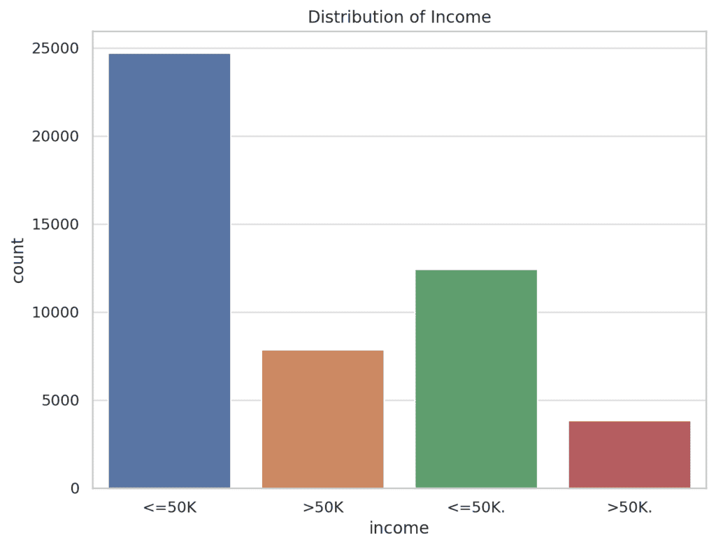
The graph below shows the distribution of the target variable income.

There are two classes: individuals earning <=50K and >50K. The majority of the individuals earn <=50K, which may indicate a somewhat imbalanced dataset.

Distribution of Numerical Features

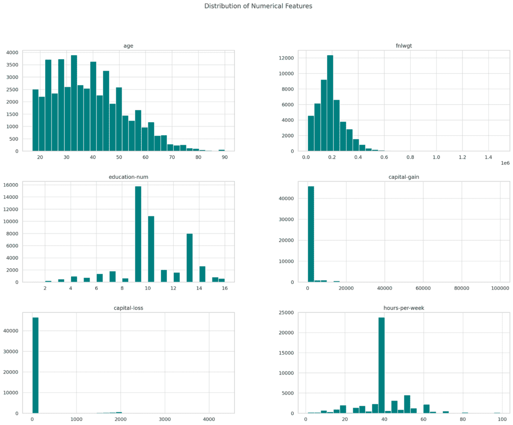
The bar charts below shows the distribution of the numerical features in the dataset. These include:

• age: Most individuals are in the working-age group.
  
• education-num: The distribution shows different levels of educational attainment.
  
• capital-gain and capital-loss: These distributions are highly skewed, with many individuals having zero gains or losses.
  
• hours-per-week: Most individuals work between 35-45 hours per week.

Summary Statistics

The summary statistics for the numerical features in the dataset are as follows:

1. Age: The average age is approximately 38.64 years, with a standard deviation of 13.71 years. The youngest individual is 17 years old, and the oldest is 90 years old.
2. Capital-gain: The mean capital gain is 1079, but the distribution is highly skewed, with a few individuals having very high capital gains (up to 99,999).
3. Capital-loss: Similar to capital-gain, capital-loss has a mean of 87.5, but most individuals have no capital loss, as indicated by the 25th, 50th, and 75th percentiles being zero.
4. Hours-per-week: The average number of hours worked per week is around 40.42, with a standard deviation of 12.39. Most individuals work a standard full-time week (40 hours).

Metric	Age	Capital-gain	Capital-loss	Hours-per-week
Mean	39	1079	88	40
Std	14	7452	403	12
Min	17	0	0	1
Max	90	99999	4356	99

Missing Values

The dataset has missing values in the following columns:

• workclass: 963 missing values
• occupation: 966 missing values
• native-country: 274 missing values

Data Cleaning

The dataset has been thoroughly cleaned and pre-processed as follows:

1. Missing Values: Missing values in the workclass, occupation, and native-country columns have been filled using the most frequent value for each column.
   
2. Encoding Categorical Variables: All categorical variables have been converted into numerical format using Label Encoding.
   
3. Outlier Detection and Removal: Outliers were identified using z-scores and removed, which reduced the dataset from 48,842 entries to 45,112 entries.
   
4. Feature Scaling: All features have been standardised using StandardScaler to ensure they are on a similar scale.
   
5. Removing Duplicates: The dataset was checked for and cleaned of any duplicate rows.

The cleaned dataset now consists of 45,112 entries and 15 standardised numerical features, making it ready for any subsequent analysis or modelling tasks.

Predictive analytics

We’ll now train a Random Forest classifier to predict whether an individual earns more than $50K annually. See the python script above for this prediction.

Random Forest Model Results

The Random Forest model was trained and evaluated on the cleaned dataset. Here are the results:

Confusion Matrix

• The confusion matrix shows how the predictions are distributed across the actual classes.

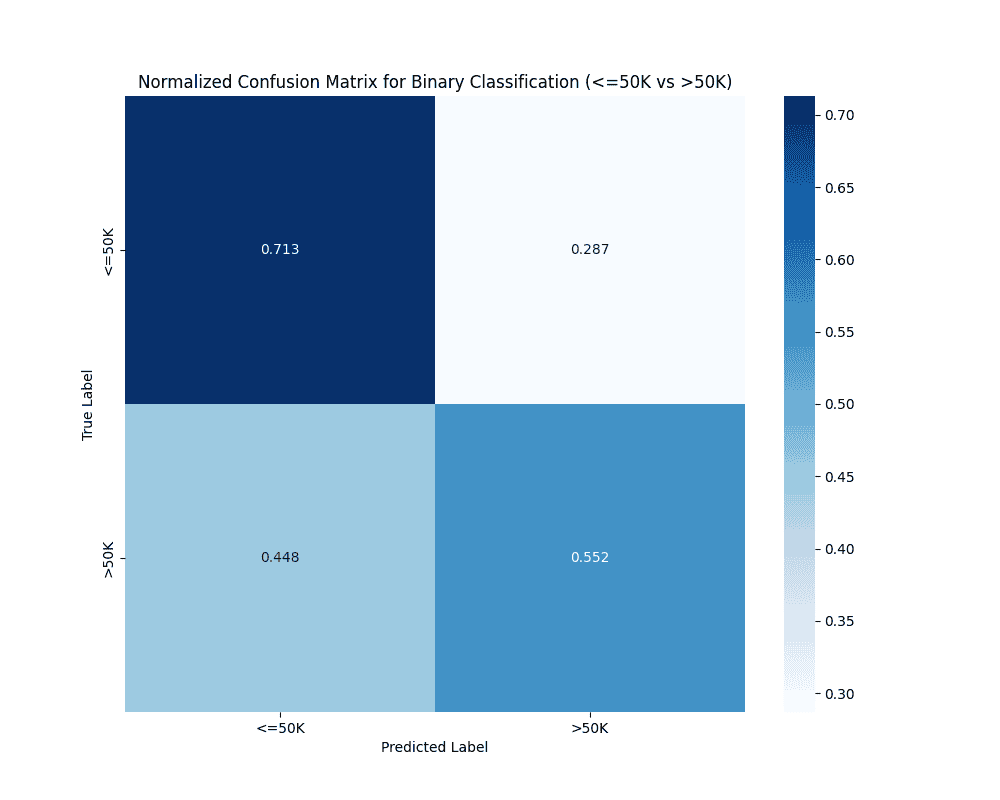
• The matrix shows that the model is better at predicting <=50K correctly (71.3%) compared to predicting >50K correctly (55.2%).
• However, it also makes a considerable number of errors, especially in predicting >50K earners, as shown by the 44.8% false negatives.

Classification Report

• Accuracy: As could be seen, the model correctly predicted whether a person makes over 50K a year about 64% of the time.
• Precision: Varies across classes, with class 0 (making ≤50K) having the highest precision at 0.60.
• Recall: The recall is relatively higher for class 0 (making ≤50K), indicating the model is better at identifying individuals making ≤50K.
• F1-Score: This score, which balances precision and recall, is highest for class 0 (making ≤50K), at 0.69.

	Precision	Recall	F1 score	Support
0	0.63	0.71	0.67	7026
1	0.64	0.55	0.59	6508
Accuracy	0.64			13534
Macro Avg	0.64	0.63	0.63	13534
Weighted Avg	0.64	0.64	0.63	13534

ROC ( Receiver Operating Characteristic) Curve

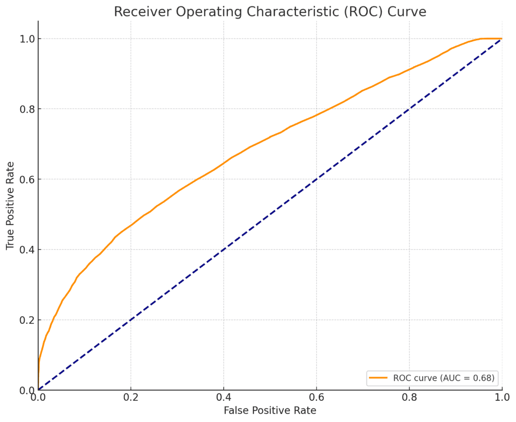
Here is the ROC curve for predicting whether a person makes over 50K a year using the Random Forest algorithm.

The AUC (Area Under the Curve) value provides a measure of how well the model distinguishes between the two classes (≤50K and >50K).

Explanation of the ROC Curve

The ROC curve is a powerful tool used to evaluate the performance of a binary classification model.

In this context, the ROC curve helps us understand how well the Random Forest model distinguishes between individuals who earn more than $50K a year (>50K) and those who do not (<=50K).

• The AUC is a single scalar value that summarises the performance of the classifier across all thresholds.
• AUC = 1.0: Perfect classification.
• AUC = 0.5: No discrimination capability (equivalent to random guessing).
• AUC < 0.5: Worse than random guessing (indicates potential issues with the model or data).

Shape of the Curve: The curve plotted for the Random Forest model tends to bow towards the top left, which indicates that the model performs better than random guessing.

However, the degree of curvature can give insight into the overall performance.

AUC Value: The AUC value of 0.68 reported on the curve indicates the overall ability of the model to distinguish between the two classes.

The closer the AUC is to 1, the better the model’s performance.

Summary of Income Levels

The model’s accuracy and performance metrics suggest that there is room for improvement.

In summary, the ROC curve and its AUC value provide a comprehensive picture of the model’s ability to differentiate between individuals who earn >50K and those who earn <=50K.

The higher the AUC, the more confident you can be in the model’s predictions. If the AUC is closer to 1, it suggests that the model is very effective at classifying individuals correctly.

If the AUC is closer to 0.5, it suggests the model is only as good as random guessing.

Perhaps model refinement through more hyperparameter tuning, feature engineering, or collecting more data that comprehensively represent the income situation may improve the model further.

Conclusion

Our exploration of the “Adult Census Income” dataset reveals the potential of machine learning in predicting income levels with reasonable accuracy.

The predictive analysis highlighted the model’s ability to differentiate between individuals earning more or less than $50K, with an ROC curve providing a clear visual representation of the model’s effectiveness.

While the model showed promise, it also underscored the challenges inherent in classification tasks, particularly when dealing with imbalanced datasets.

The accuracy and classification metrics indicate that while the model performs well in some areas, there is room for improvement.

This is could be achieved through more sophisticated feature engineering or hyperparameter tuning.

Reference

Becker,Barry and Kohavi,Ronny. (1996). Adult. UCI Machine Learning Repository. https://doi.org/10.24432/C5XW20.